Resampled PSFs from JWST/NIRCam Imaging
This example notebook shows how spike interacts with JWST/NIRCam imaging to generate a resampled PSF. This notebook uses observations from “PANORAMIC – A Pure Parallel Wide Area Legacy Imaging Survey at 1-5 Micron” (PI: Dr. Christina Williams):
jw02514162001_03201_00001_nrca2_cal.fits
jw02514162001_03201_00002_nrca2_cal.fits
jw02514162001_03201_00003_nrca2_cal.fits
The easiest way to find these data in the MAST archive is by searching for observation IDs jw02514162001_03201_00001_nrca2, jw02514162001_03201_00002_nrca2, jw02514162001_03201_00003_nrca2. spike uses calibrated, but not-yet co-added images (i.e., “Level 2” data products), so be sure that your download includes ‘cal’ files.
These data are also available here.
NOTE: Environment variables are not always read in properly within Jupyter notebooks/JupyterLab – see here for some additional details of how to access them.
Initial setup and visualization
[ ]:
from spike.psf import jwst # import the relevant top-level module from spike

datapath = '/path/to/nircam/data'
outputpath = 'psfs' #default is /psfs, defined from your working directory
Note that if you choose to create resampled PSFs for the same data and object location using multiple PSF generation methods, you will want to define a new ‘savedir’ each time to avoid conflicts between files with the same name.
We’ll also define an object – in this case, a set of coordinates – for which the PSF will be generated.
[2]:
obj = '10:00:33.588 +02:10:24.18' #can also be a resolvable name or coordinates in decimal degrees
Now, we can call spike.psf.jwst – as an initial example we’ll use the most minimal inputs. By default, in addition to saving drizzled PSFs and any intermediate products in the directory given by ‘savedir’ (here the argument will be the outputpath variable we defined), this function will return a dictionary that stores model PSFs indexed by filter and object.
If returnpsf = 'full' (default), the arrays in the dictionary will be the full drizzled image field of view. If returnpsf = 'crop', the arrays in the dictionary will be the cutout region around the object location with the size of the cutout determined by the ‘cutout_fov’ argument; the cropped region around the drizzled PSF will also be saved as a FITS file, including its WCS information (can be toggled off with savecutout = False).
spike assumes that the input files have not yet been “tweaked” and handles that step for you. If your input images have been tweaked or if you would like to skip this step for other reasons, specify pretweaked = True in calling spike.psf.jwst. The JWST pipeline replaces the suffix of the tweaked files, going from ‘cal’ to ‘tweakregstep’, if you tweak the files with spike. As such, in addition to pretweaked = True, it will be necessary to set img_type = 'tweakregstep'.
The examples in this notebook follow this convention.
The outputs can be very long due to all of the print statements from the tweak, PSF generation, and resampling steps. Outputs have been cleared for cells where spike.psf.jwst was run.
[ ]:
dpsf = jwst(img_dir = datapath, obj = obj, img_type = 'cal', inst = 'NIRCam',
           savedir = outputpath, pretweaked = False)
In this case dpsf will be very simple, since we are only looking at one set of coordinates and one filter:
[4]:
dpsf
[4]:
{'10:00:33.588 +02:10:24.18': {'F115W': array([[nan, nan, nan, ..., nan, nan, nan],
         [nan, nan, nan, ..., nan, nan, nan],
         [nan, nan, nan, ..., nan, nan, nan],
         ...,
         [nan, nan, nan, ..., nan, nan, nan],
         [nan, nan, nan, ..., nan, nan, nan],
         [nan, nan, nan, ..., nan, nan, nan]],
        shape=(2080, 2077), dtype='>f4')}}
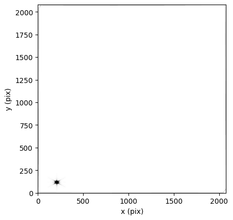
spike can automatically plot model PSFs as they are generated, and generates PSFs regardless of whether they are plotted (or returned). To show the output drizzled PSFs here, we will plot them directly. Therefore, we will import matplotlib below. Since returnpsf = 'full' by default, the array stored in dpsf shows the drizzled PSF in the context of the entire co-added image footprint. This is equivalent to reading in the image stored in ‘100031+021026_F115W_resamplestep.fits’.
[5]:
import matplotlib.pyplot as plt
import numpy as np

dat = dpsf['10:00:33.588 +02:10:24.18']['F115W']

fig = plt.figure()
plt.imshow(dat, vmin = np.nanpercentile(dat[dat != 0], 20), vmax = np.nanpercentile(dat[dat != 0], 97),
            origin = 'lower', cmap = 'Greys')
plt.xlabel('x (pix)')
plt.ylabel('y (pix)')
[5]:
Text(0, 0.5, 'y (pix)')
We can index the array to just show the PSF below:
[6]:
dat = dpsf['10:00:33.588 +02:10:24.18']['F115W'][49: 189, 140:280]

fig = plt.figure()
plt.imshow(dat, vmin = np.nanpercentile(dat[dat != 0], 20), vmax = np.nanpercentile(dat[dat != 0], 97),
            origin = 'lower', cmap = 'Greys', extent = [140, 280, 49, 189])
plt.xlabel('x (pix)')
plt.ylabel('y (pix)')
[6]:
Text(0, 0.5, 'y (pix)')

PSF generation methods
By default, PSFs are generated for spike.psf.jwst by STPSF (formerly WebbPSF) for a 6 arcsec x 6 arcsec region; users have complete control over the specifics of the PSF generation with keyword arguments for spike.psfgen.jwpsf and the optional dictionary calckwargs which is a keyword argument for spike.psf.jwst and feeds additional keyword arguments to STPSF (WebbPSF) when it’s called by spike. This is true across methods: to change the parameters within a
method (e.g., updating model arguments, setting different detection thresholds for the empirical PSFs, …), spike.psf.jwst directly takes keyword arguments for the specified ‘method’. Details of allowed arguments are available in the spike.psfgen documentation.
One advantage of spike is that it can be used flexibly with a variety of different PSF generation methods – to change which one is used, simply use the ‘method’ argument. Built-in options are:
‘WebbPSF’ (this name is maintained in
spikein lieu ofSTPSFto avoid confusion with the empirical STDPSFs)‘STDPSF’
‘epsf’
‘PSFEx’
If method = 'USER', then the keyword argument ‘usermethod’ must also be specified, pointing to either a function or a directory that houses model PSFs that follow the [imgprefix]_[coords]_[band]_psf.fits, e.g., imgprefix_23.31+30.12_F814W_psf.fits or imgprefix_195.78-46.52_F555W_psf.fits naming scheme.
We’ll use STDPSFs below.
[ ]:
dpsf = jwst(img_dir = datapath, obj = obj, img_type = 'tweakregstep', inst = 'NIRCam',
           method = 'STDPSF', savedir = outputpath, pretweaked = True)
[8]:
dpsf
[8]:
{'10:00:33.588 +02:10:24.18': {'F115W': array([[nan, nan, nan, ..., nan, nan, nan],
         [nan, nan, nan, ..., nan, nan, nan],
         [nan, nan, nan, ..., nan, nan, nan],
         ...,
         [nan, nan, nan, ..., nan, nan, nan],
         [nan, nan, nan, ..., nan, nan, nan],
         [nan, nan, nan, ..., nan, nan, nan]],
        shape=(2080, 2077), dtype='>f4')}}
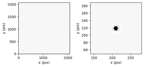
[9]:
dat = dpsf['10:00:33.588 +02:10:24.18']['F115W']
datcrop = dpsf['10:00:33.588 +02:10:24.18']['F115W'][49: 189, 140:280]

fig, ax = plt.subplots(1, 2, gridspec_kw = {'wspace':0.4})
ax[0].imshow(dat, vmin = np.nanpercentile(dat[dat != 0], 20), vmax = np.nanpercentile(dat[dat != 0], 90),
            origin = 'lower', cmap = 'Greys')
ax[0].set_xlabel('x (pix)')
ax[0].set_ylabel('y (pix)')

ax[1].imshow(datcrop, origin = 'lower', cmap = 'Greys', extent = [140, 280, 49, 189],
             vmin = np.nanpercentile(datcrop[datcrop != 0], 20),
             vmax = np.nanpercentile(datcrop[datcrop != 0], 90))
ax[1].set_xlabel('x (pix)')
ax[1].set_ylabel('y (pix)')
[9]:
Text(0, 0.5, 'y (pix)')
Generating multiple PSFs, automatic cropping
spike can also be used to generate PSFs for multiple objects/coordinates simultaneously. We’ll do this using the default STPSF parameters below.
[ ]:
obj = ['10:00:33.588 +02:10:24.18', '10:00:31.0132 +02:09:53.23']

dpsf = jwst(img_dir = datapath, obj = obj, img_type = 'tweakregstep', inst = 'NIRCam',
           savedir = outputpath, pretweaked = True, returnpsf = 'crop')
[11]:
dpsf
[11]:
{'10:00:33.588 +02:10:24.18': {'F115W': array([[1.7523478e-08, 1.5072770e-08, 1.6001122e-08, ..., 4.5324740e-08,
          4.0344979e-08, 3.7317228e-08],
         [2.0585176e-08, 1.8902893e-08, 1.8593946e-08, ..., 4.6495114e-08,
          4.2483450e-08, 4.4546880e-08],
         [2.1103494e-08, 2.1986096e-08, 2.2065652e-08, ..., 4.7852630e-08,
          4.7637034e-08, 5.0260066e-08],
         ...,
         [3.4837679e-08, 3.2755768e-08, 2.9932966e-08, ..., 1.9081225e-08,
          1.9336706e-08, 1.8856179e-08],
         [3.1081413e-08, 2.8494831e-08, 2.6283381e-08, ..., 2.1312930e-08,
          1.8516369e-08, 1.8506489e-08],
         [2.8021878e-08, 2.5805665e-08, 2.3233691e-08, ..., 2.6041441e-08,
          2.0895374e-08, 1.8359176e-08]], shape=(151, 151), dtype='>f4')},
 '10:00:31.0132 +02:09:53.23': {'F115W': array([[1.4725797e-08, 1.5325554e-08, 1.5904833e-08, ..., 4.0547768e-08,
          3.6523286e-08, 3.9292836e-08],
         [1.8591647e-08, 1.7337449e-08, 1.7776829e-08, ..., 4.2939519e-08,
          4.1410200e-08, 4.9462614e-08],
         [2.0925048e-08, 2.0995257e-08, 2.0178003e-08, ..., 4.5266223e-08,
          5.3111801e-08, 6.0602673e-08],
         ...,
         [3.4067924e-08, 3.0034233e-08, 2.5755600e-08, ..., 1.8544458e-08,
          1.8454607e-08, 1.6817625e-08],
         [2.9443605e-08, 2.4505031e-08, 2.3776957e-08, ..., 1.8345480e-08,
          1.8026803e-08, 1.7597836e-08],
         [2.3228850e-08, 2.2441288e-08, 2.5477370e-08, ..., 2.1925183e-08,
          1.7846531e-08, 1.7543138e-08]], shape=(151, 151), dtype='>f4')}}
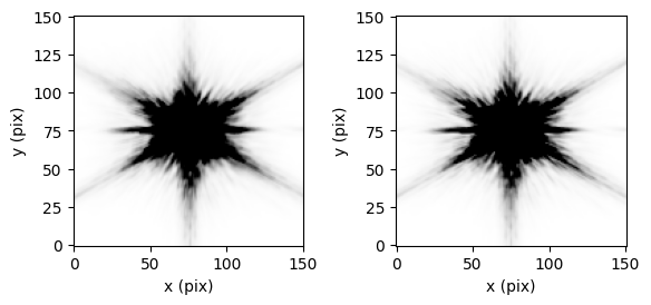
Since we’ve selected returnpsf = 'crop', the output array is already cropped to the immediate region around the PSF. Selecting both returnpsf = 'crop' and savecutout = True (default), will save a FITS file that stores the cropped resampled PSF – the name is the same as the for the full saved image with ‘_crop’ appended.
[13]:
dat = dpsf['10:00:33.588 +02:10:24.18']['F115W']

fig, ax = plt.subplots(1, 2, gridspec_kw = {'wspace':0.4})
ax[0].imshow(dat, vmin = np.nanpercentile(dat[dat != 0], 20), vmax = np.nanpercentile(dat[dat != 0], 90),
            origin = 'lower', cmap = 'Greys')
ax[0].set_xlabel('x (pix)')
ax[0].set_ylabel('y (pix)')

dat = dpsf['10:00:31.0132 +02:09:53.23']['F115W']

ax[1].imshow(dat, vmin = np.nanpercentile(dat[dat != 0], 20), vmax = np.nanpercentile(dat[dat != 0], 90),
            origin = 'lower', cmap = 'Greys',)
ax[1].set_xlabel('x (pix)')
ax[1].set_ylabel('y (pix)')
[13]:
Text(0, 0.5, 'y (pix)')